Currency Relative Strengths V.2 [GM]Version 2 Updates
Speed has been increased by ~7X
Highest and lowest pairs now highlighted using brighter colors
Re-ordered pairs from highest to lowest 'flight to risk' rating
I created this tool for the purpose of determining strongest and weakest currencies over different periods of time. Each major currency is compared to the field of other majors and its average change is measured over a predetermined period of time. The result is displayed as a percentage. I use it for trend following but it can also be used to fade exhaustion.
Instructions
Add indicator to chart
Select a time frame under settings
Place cursor over period of interest
Click "Data Window" on right hand side bar
View % change avg values for each currency
Cari skrip untuk "relative strength"

Relative Momentum Index The Relative Momentum Index (RMI) was developed by Roger Altman. Impressed
with the Relative Strength Index's sensitivity to the number of look-back
periods, yet frustrated with it's inconsistent oscillation between defined
overbought and oversold levels, Mr. Altman added a momentum component to the RSI.
As mentioned, the RMI is a variation of the RSI indicator. Instead of counting
up and down days from close to close as the RSI does, the RMI counts up and down
days from the close relative to the close x-days ago where x is not necessarily
1 as required by the RSI). So as the name of the indicator reflects, "momentum" is
substituted for "strength".

EDUVEST Lorentzian ClassificationEDUVEST Lorentzian Classification - Machine Learning Signal Detection
━━━━━━━━━━━━━━━━━━━━━━━━━━━━━━━━━━━━━━━━━━━━━━━━
█ ORIGINALITY
This indicator enhances the original Lorentzian Classification concept by jdehorty with EduVest's visual modifications and alert system integration. The core innovation is using Lorentzian distance instead of Euclidean distance for k-NN classification, providing more robust pattern recognition in financial markets.
━━━━━━━━━━━━━━━━━━━━━━━━━━━━━━━━━━━━━━━━━━━━━━━━
█ WHAT IT DOES
- Generates BUY/SELL signals using machine learning classification
- Displays kernel regression estimate for trend visualization
- Shows prediction values on each bar
- Provides trade statistics (Win Rate, W/L Ratio)
- Includes multiple filter options (Volatility, Regime, ADX, EMA, SMA)
━━━━━━━━━━━━━━━━━━━━━━━━━━━━━━━━━━━━━━━━━━━━━━━━
█ HOW IT WORKS
【Lorentzian Distance Calculation】
Unlike Euclidean distance, Lorentzian distance uses logarithmic transformation:
d = Σ log(1 + |xi - yi|)
This provides:
- Better handling of outliers
- More stable distance measurements
- Reduced sensitivity to extreme values
【Feature Engineering】
The classifier uses up to 5 configurable features:
- RSI (Relative Strength Index)
- WT (WaveTrend)
- CCI (Commodity Channel Index)
- ADX (Average Directional Index)
Each feature is normalized using the n_rsi, n_wt, n_cci, or n_adx functions.
【k-Nearest Neighbors Classification】
1. Calculate Lorentzian distance between current bar and historical bars
2. Find k nearest neighbors (default: 8)
3. Sum predictions from neighbors
4. Generate signal based on prediction sum (>0 = Long, <0 = Short)
【Kernel Regression】
Uses Rational Quadratic kernel for smooth trend estimation:
- Lookback Window: 8
- Relative Weighting: 8
- Regression Level: 25
【Filters】
- Volatility Filter: Filters signals during extreme volatility
- Regime Filter: Identifies market regime using threshold
- ADX Filter: Confirms trend strength
- EMA/SMA Filter: Trend direction confirmation
━━━━━━━━━━━━━━━━━━━━━━━━━━━━━━━━━━━━━━━━━━━━━━━━
█ HOW TO USE
【Recommended Settings】
- Timeframe: 15M, 1H, 4H, Daily
- Neighbors Count: 8 (default)
- Feature Count: 5 for comprehensive analysis
【Signal Interpretation】
- Green BUY label: Long entry signal
- Red SELL label: Short entry signal
- Bar colors: Green (bullish) / Red (bearish) prediction strength
【Trade Statistics Panel】
- Winrate: Historical win percentage
- Trades: Total (Wins|Losses)
- WL Ratio: Win/Loss ratio
- Early Signal Flips: Premature signal changes
【Filter Recommendations】
- Enable Volatility Filter for ranging markets
- Enable Regime Filter for trend confirmation
- Use EMA Filter (200) for higher timeframes
━━━━━━━━━━━━━━━━━━━━━━━━━━━━━━━━━━━━━━━━━━━━━━━━
█ CREDITS
Original Lorentzian Classification concept and MLExtensions library by jdehorty.
Enhanced with visual modifications and alert integration by EduVest.
License: Mozilla Public License 2.0

BAVC (Clone) Rolling Curves, Peak MarkersBAVC (Clone) — Rolling Curves + Peak Markers
BAVC (Clone) is a volume-based momentum and participation indicator designed to visualize aggressive buying vs aggressive selling pressure using rolling volume curves and structural peak detection.
This script is a functional clone of a Bid/Ask Volume Curve concept, implemented using approximated volume splitting (uptick/downtick or close vs open) so it works on standard TradingView data without requiring true bid/ask feeds.
What the Indicator Shows
1. Rolling Buy & Sell Volume Curves
Volume is split into Buy (aggressive buyers) and Sell (aggressive sellers) using a selectable approximation method.
Each side is accumulated over a configurable lookback window.
Optional EMA smoothing is applied to reduce noise and highlight participation trends.
Interpretation:
Rising Buy Curve → increasing buyer dominance
Rising Sell Curve → increasing seller dominance
Expanding separation → stronger directional conviction
Convergence / flattening → balance, absorption, or transition
2. Adaptive Color Intensity (Optional)
Curve opacity can remain fixed or
Automatically adapt based on relative dominance strength
Stronger imbalances visually stand out without adding extra indicators
3. Structural Peak & Trough Detection
The script identifies significant local extremes in both curves:
Buy-side peaks & troughs
Sell-side peaks & troughs
Each peak is filtered using:
Swing width (bars left/right)
Relative strength vs recent maximum
Minimum depth for troughs
Markers can be displayed as:
Circles directly on the curves, or
Minimal labels (▲ / ▼)
Interpretation:
Buy-side highs → possible exhaustion or distribution
Buy-side lows → loss of initiative / absorption
Sell-side highs → aggressive selling climax
Sell-side lows → selling pressure weakening
4. Alerts
Optional alerts fire when:
A significant Buy-side peak forms
A significant Buy-side trough forms
A significant Sell-side peak forms
A significant Sell-side trough forms
These are intended as contextual signals, not standalone trade triggers.
5. Status Line Helper
An optional real-time status label displays:
Lookback settings
Current rolling Buy and Sell volume sums
This is useful for quick confirmation without opening the settings panel.
Important Notes
This indicator uses volume behavior, not price.
It is best used as a confirmation tool alongside:
Structure
Time-based context
VWAP / trend filters
It does not generate buy or sell signals by itself.
Best Use Cases
Spotting institutional participation
Confirming trend strength or exhaustion
Identifying absorption before reversals
Filtering low-quality entries during choppy periods

Refined Liquidity Flow IndicatorRefined Liquidity Flow Indicator - How It Works
The Refined Liquidity Flow Indicator is designed to help traders identify the flow of liquidity into and out of the market based on multiple technical factors. It combines price movement, market sentiment, volatility, and volume to give a comprehensive view of market conditions. The indicator gives buy and sell signals by calculating the flow of liquidity based on these factors.
Key Components of the Indicator:
Liquidity Flow Calculation:
The core of the indicator is the liquidity flow calculation, which is based on several factors:
Liquidity Flow=(V×ΔP)+(α×ATR)+(β×RSI)+(γ×ΔP)
Where:
𝑉 is the volume (the amount of trading activity).
ΔP is the price change (the difference between the current and previous closing price).
ATR (Average True Range) is used to measure market volatility.
RSI (Relative Strength Index) reflects market sentiment.
𝛼 𝛽 𝛾
are adjustable weights (parameters) that allow you to control how much influence each factor has on the liquidity flow calculation.
Key Indicators:
Volume (V): The amount of trades occurring in the market. A high volume indicates more activity, which is essential for confirming liquidity flow.
Price Change (ΔP): The difference between the current price and the previous price, which helps assess the strength and direction of the market move.
ATR (Average True Range): A measure of market volatility, indicating how much the price fluctuates over a specified period. A higher ATR suggests greater volatility, which often corresponds with a greater flow of liquidity.
RSI (Relative Strength Index): A momentum oscillator that measures whether a market is overbought or oversold. The RSI can help determine whether the market sentiment is bullish or bearish.
How to Use the Indicator:
Set Up: After adding the Refined Liquidity Flow Indicator to your chart, you can adjust the following settings directly from the indicator's settings panel:
α: Weight for volatility (ATR).
β: Weight for market sentiment (RSI).
γ: Weight for price change.
ATR Length: Customize the period for the ATR.
RSI Length: Customize the period for the RSI.
SMA Length: Customize the period for the Simple Moving Average.
Interpreting Signals:
Green Signal (Liquidity In): Indicates that liquidity is entering the market. This often signals a potential buy opportunity when the price is moving upwards with strong volume and market sentiment.
Red Signal (Liquidity Out): Indicates that liquidity is leaving the market. This typically signals a potential sell opportunity when the price is moving downwards with strong volume and market sentiment.
Fine-Tuning for Your Strategy:
By adjusting the weights and the lengths of the indicators, you can fine-tune the indicator to match your trading style. For example, if you want to give more weight to price movements, you can increase γ. If you want to focus more on market sentiment, adjust β.

Bitcoin vs. S&P 500 Performance Comparison**Full Description:**
**Overview**
This indicator provides an intuitive visual comparison of Bitcoin's performance versus the S&P 500 by shading the chart background based on relative strength over a rolling lookback period.
**How It Works**
- Calculates percentage returns for both Bitcoin and the S&P 500 (ES1! futures) over a specified lookback period (default: 75 bars)
- Compares the returns and shades the background accordingly:
- **Green/Teal Background**: Bitcoin is outperforming the S&P 500
- **Red/Maroon Background**: S&P 500 is outperforming Bitcoin
- Displays a real-time performance difference label showing the exact percentage spread
**Key Features**
✓ Rolling performance comparison using customizable lookback period (default 75 bars)
✓ Clean visual representation with adjustable transparency
✓ Works on any timeframe (optimized for daily charts)
✓ Real-time performance differential display
✓ Uses ES1! (E-mini S&P 500 continuous futures) for accurate comparison
✓ Fine-tuning adjustment factor for precise calibration
**Use Cases**
- Identify market regimes where Bitcoin outperforms or underperforms traditional equities
- Spot trend changes in relative performance
- Assess risk-on vs risk-off periods
- Compare Bitcoin's momentum against broader market conditions
- Time entries/exits based on relative strength shifts
**Settings**
- **S&P 500 Symbol**: Default ES1! (can be changed to SPX or other indices)
- **Lookback Period**: Number of bars for performance calculation (default: 75)
- **Adjustment Factor**: Fine-tune calibration to match specific data feeds
- **Transparency Controls**: Customize background shading intensity
- **Show/Hide Label**: Toggle performance difference display
**Best Practices**
- Use on daily timeframe for swing trading and position analysis
- Combine with other momentum indicators for confirmation
- Watch for color transitions as potential regime change signals
- Consider using multiple timeframes for comprehensive analysis
**Technical Details**
The indicator calculates rolling percentage returns using the formula: ((Current Price / Price ) - 1) × 100, then compares Bitcoin's return to the S&P 500's return over the same period. The background color dynamically updates based on which asset is showing stronger performance.

Distance Dashboard (50DMA / 52W High / 20DMA)Distance Dashboard – Summary
The Distance Dashboard indicator provides a quick snapshot of where price is positioned relative to three key reference points:
Distance of current HIGH from the 50-day moving average (50DMA)
Helps gauge how extended price is above or below medium-term trend support.
Distance of current LOW from the 52-week HIGH
Shows how far price has pulled back from long-term highs.
Distance of current HIGH from the 20-day moving average (20DMA)
Measures short-term extension and potential overbought/overextended behaviour.
The indicator displays these values in a clean, movable table directly on the price chart.
It does not affect chart scaling and is designed for quick visual assessment of trend extension and relative strength.

Normalised Volume Oscillator [BackQuant]Normalised Volume Oscillator
A refined evolution of the Klinger Volume Oscillator, rebuilt for clarity, precision, and adaptability. This tool normalizes volume-driven momentum into a bounded scale so you can easily identify shifts in accumulation and distribution across any asset or timeframe, while keeping readings comparable between markets.
What this indicator does
The Normalised Volume Oscillator quantifies the balance between buying and selling pressure using the Klinger Volume Oscillator (KVO) as its base, then rescales it dynamically into a normalized range between -0.5 and +0.5. This normalization allows traders to interpret relative strength and exhaustion in volume flow, rather than dealing with raw unbounded values that differ across symbols.
It is a momentum-volume hybrid that reveals the strength of trend participation: when buyers dominate, normalized readings rise toward +0.5; when sellers dominate, they fall toward -0.5. The midline (0) acts as an equilibrium between accumulation and distribution.
Core components
Klinger Volume Oscillator: The foundation of this indicator, combining volume with price trend direction to measure long-term money flow relative to short-term movement.
Normalization process: The raw KVO is scaled over a user-defined Normalisation Period , computing `(KVO - lowest) / (highest - lowest) - 0.5`. This centers all readings around zero, allowing overbought/oversold detection independent of asset volatility or volume magnitude.
Signal moving average: The normalized KVO is smoothed with a user-selectable moving average type—SMA, EMA, DEMA, TEMA, HMA, ALMA, and others. This becomes the signal line for confirmation of trend direction or mean-reversion setups.
How it works conceptually
1. The KVO detects when volume supports price movement (bullish) or diverges from it (bearish).
2. The script normalizes the raw KVO so that relative magnitude is consistent—what is “strong buying pressure” looks the same on BTCUSD as it does on AAPL.
3. Overbought and oversold regions are derived statistically, rather than from arbitrary values, based on percentile zones around ±0.4 and ±0.5.
4. The oscillator is optionally combined with a moving average to help identify crossovers, momentum shifts, and divergence confirmation.
How to interpret it
Above 0: Indicates dominant buying pressure and likely continuation of upward momentum.
Below 0: Suggests dominant selling pressure and potential continuation of downward movement.
Crosses of 0: Often mark transitions between accumulation and distribution phases.
+0.4 to +0.5 zone: Overbought region where buying intensity is stretched; watch for deceleration or divergence.
[-0.4 to -0.5 zone: Oversold region indicating panic or exhaustion in selling.
Signal-line crossover: A traditional momentum confirmation method; when the normalized KVO crosses above its moving average, buyers regain control, and vice versa.
Why normalization matters
Typical volume oscillators are asset-specific—what is considered “high” volume for one symbol is not the same for another. By dynamically normalizing KVO values within a rolling lookback, this version transforms raw amplitude into a standardized scale. This means you can:
Compare multiple assets objectively.
Set consistent alert thresholds for overbought/oversold regions.
Avoid misleading interpretations from absolute oscillator values.
Customization and UI
Moving Average Type & Period: Select your preferred smoothing method (SMA, EMA, TEMA, etc.) and adjust its period to tune sensitivity.
Normalisation Period: Defines how many bars the KVO range is measured over; shorter periods adapt faster, longer ones smooth more.
Visual Toggles:
* Show Oscillator : enables or hides the core histogram.
* Show Moving Average : adds a smoothed overlay for signal confirmation.
* Paint Candles : optional color overlay for chart candles based on oscillator direction.
* Show Static Levels : displays ±0.4 and ±0.5 zones for overbought/oversold boundaries.
How to use it
Trend confirmation: Use midline (0) crossovers as confirmation of emerging trend shifts—cross above 0 suggests a new bullish phase, cross below 0 a bearish one.
Reversal spotting: Look for normalized readings reaching ±0.5 and flattening, or diverging against price extremes.
Divergence analysis: When price makes a new high but the normalized oscillator fails to, it signals waning buying conviction (and vice versa for lows).
Multi-timeframe integration: Works best alongside higher timeframe trend filters or moving averages; normalization makes this consistent.
Alerts
Prebuilt alert conditions allow quick automation:
Midline crossovers (0): transition between accumulation and distribution.
Overbought (+0.4) and Oversold (-0.4) triggers for potential exhaustion.
Signal moving-average crosses for confirmation entries.
Tips for use
Combine with price structure—don’t fade every overbought/oversold reading; confirm with break of structure or candle patterns.
Use longer normalization periods for position trading, shorter for intraday analysis.
In choppy markets, treat 0-line oscillations as noise filters, not trade triggers.
Summary
The Normalised Volume Oscillator modernizes the classic Klinger Volume Oscillator by normalizing its readings into a standardized range. This makes it more adaptive across assets and timeframes, improves interpretability, and provides intuitive, data-driven overbought/oversold levels. Whether used standalone or as a confirmation layer, it offers a clearer view of volume dynamics—revealing when markets are truly being accumulated, distributed, or stretched beyond their sustainable extremes.

Holt Damped Forecast [CHE]A Friendly Note on These Pine Script Scripts
Hey there! Just wanted to share a quick, heartfelt heads-up: All these Pine Script examples come straight from my own self-study adventures as a total autodidact—think late nights tinkering and learning on my own. They're purely for educational vibes, helping me (and hopefully you!) get the hang of Pine Script basics, cool indicators, and building simple strategies.
That said, please know this isn't any kind of financial advice, investment nudge, or pro-level trading blueprint. I'd love for you to dive in with your own research, run those backtests like a champ, and maybe bounce ideas off a qualified expert before trying anything in a real trading setup. No guarantees here on performance or spot-on accuracy—trading's got its risks, and those are totally on each of us.
Let's keep it fun and educational—happy coding! 😊
Holt Damped Forecast — Damped trend forecasts with fan bands for uncertainty visualization and momentum integration
Summary
This indicator applies damped exponential smoothing to generate forward price forecasts, displaying them as probabilistic fan bands to highlight potential ranges rather than point estimates. It incorporates residual-based uncertainty to make projections more reliable in varying market conditions, reducing overconfidence in strong trends. Momentum from the trend component is shown in an optional label alongside signals, aiding quick assessment of direction and strength without relying on lagging oscillators.
Motivation: Why this design?
Standard exponential smoothing often extrapolates trends indefinitely, leading to unrealistic forecasts during mean reversion or weakening momentum. This design uses damping to gradually flatten long-term projections, better suiting real markets where trends fade. It addresses the need for visual uncertainty in forecasts, helping traders avoid entries based on overly optimistic point predictions.
What’s different vs. standard approaches?
- Reference baseline: Diverges from basic Holt's linear exponential smoothing, which assumes persistent trends without decay.
- Architecture differences:
- Adds damping to the trend extrapolation for finite-horizon realism.
- Builds fan bands from historical residuals for probabilistic ranges at multiple confidence levels.
- Integrates a dynamic label combining forecast details, scaled momentum, and directional signals.
- Applies tail background coloring to recent bars based on forecast direction for immediate visual cues.
- Practical effect: Charts show converging forecast bands over time, emphasizing shorter horizons where accuracy is higher. This visibly tempers aggressive projections in trends, making it easier to spot when uncertainty widens, which signals potential reversals or consolidation.
How it works (technical)
The indicator maintains two persistent components: a level tracking the current price baseline and a trend capturing directional slope. On each bar, the level updates by blending the current source price with a one-step-ahead expectation from the prior level and damped trend. The trend then adjusts by weighting the change in level against the prior damped trend. Forecasts extend this forward over a user-defined number of steps, with damping ensuring the trend influence diminishes over distance.
Uncertainty derives from the standard deviation of historical residuals—the differences between actual prices and one-step expectations—scaled by the damping structure for the forecast horizon. Bands form around the median forecast at specified confidence intervals using these scaled errors. Initialization seeds the level to the first bar's price and trend to zero, with persistence handling subsequent updates. A security call fetches the last bar index for tail logic, using lookahead to align with realtime but introducing minor repaint on unconfirmed bars.
Parameter Guide
The Source parameter selects the price input for level and residual calculations, defaulting to close; consider using high or low for assets sensitive to volatility, as close works well for most trend-following setups. Forecast Steps (h) defines the number of bars ahead for projections, defaulting to 4—shorter values like 1 to 5 suit intraday trading, while longer ones may widen bands excessively in choppy conditions. The Color Scheme (2025 Trends) option sets the base, up, and down colors for bands, labels, and backgrounds, starting with Ruby Dawn; opt for serene schemes on clean charts or vibrant ones to stand out in dark themes.
Level Smoothing α controls the responsiveness of the price baseline, defaulting to 0.3—values above 0.5 enhance tracking in fast markets but may amplify noise, whereas lower settings filter disturbances better. Trend Smoothing β adjusts sensitivity to slope changes, at 0.1 by default; increasing to 0.2 helps detect emerging shifts quicker, but keeping it low prevents whipsaws in sideways action. Damping φ (0..1) governs trend persistence, defaulting to 0.8—near 0.9 preserves carryover in sustained moves, while closer to 0.5 curbs overextensions more aggressively.
Show Fan Bands (50/75/95) toggles the probabilistic range display, enabled by default; disable it in oscillator panes to reduce clutter, but it's key for overlay forecasts. Residual Window (Bars) sets the length for deviation estimates, at 400 bars initially—100 to 200 works for short timeframes, and 500 or more adds stability over extended histories. Line Width determines the thickness of band and median lines, defaulting to 2; go thicker at 3 to 5 for emphasis on higher timeframes or thinner for layered indicators.
Show Median/Forecast Line reveals the central projection, on by default—hide if bands provide enough detail, or keep for pinpoint entry references. Show Integrated Label activates the combined view of forecast, momentum, and signal, defaulting to true; it's right-aligned for convenience, so turn it off on smaller screens to save space. Show Tail Background colors the last few bars by forecast direction, enabled initially; pair low transparency for subtle hints or higher for bolder emphasis.
Tail Length (Bars) specifies bars to color backward from the current one, at 3 by default—1 to 2 fits scalping, while 5 or more underscores building momentum. Tail Transparency (%) fades the background intensity, starting at 80; 50 to 70 delivers strong signals, and 90 or above allows seamless blending. Include Momentum in Label adds the scaled trend value, defaulting to true—ATR% scaling here offers relative strength context across assets.
Include Long/Short/Neutral Signal in Label displays direction from the trend sign, on by default; neutral helps in ranging markets, though it can be overlooked during strong trends. Scaling normalizes momentum output (raw, ATR-relative, or level-relative), set to ATR% initially—ATR% ensures cross-asset comparability, while %Level provides percentage perspectives. ATR Length defines the period for true range averaging in scaling, at 14; align it with your chart timeframe or shorten for quicker volatility responses.
Decimals sets precision in the momentum label, defaulting to 2—0 to 1 yields clean integers, and 3 or more suits detailed forex views. Show Zero-Cross Markers places arrows at direction changes, enabled by default; keep size small to minimize clutter, with text labels for fast scanning.
Reading & Interpretation
Fan bands expand outward from the current bar, with the median line as the central forecast—narrower bands indicate lower uncertainty, wider suggest caution. Colors tint up (positive forecast vs. prior level) in the scheme's up hue and down otherwise. The optional label lists the horizon, median, and range brackets at 50%, 75%, and 95% levels, followed by momentum (scaled per mode) and signal (Long if positive trend, Short if negative, Neutral if zero). Zero-cross arrows mark trend flips: upward triangle below bar for bullish cross, downward above for bearish. Tail background reinforces the forecast direction on recent bars.
Practical Workflows & Combinations
- Trend following: Enter long on upward zero-cross if median forecast rises above price and bands contain it; confirm with higher highs/lows. Short on downward cross with falling median.
- Exits/Stops: Trail stops below 50% lower band in longs; exit if momentum drifts negative or signal turns neutral. Use wider bands (75/95%) for conservative holds in volatile regimes.
- Multi-asset/Multi-TF: Defaults work across stocks, forex, crypto on 5m-1D; scale steps by TF (e.g., 10+ on daily). Layer with volume or structure tools—avoid over-reliance on isolated crosses.
Behavior, Constraints & Performance
Closed-bar logic ensures stable historical plots, but realtime updates via security lookahead may shift forecasts until bar confirmation, introducing minor repaint on the last bar. No explicit HTF calls beyond bar index fetch, minimizing gaps but watch for low-liquidity assets. Resources include a 2000-bar lookback for residuals and up to 500 labels, with no loops—efficient for most charts. Known limits: Early bars show wide bands due to sparse residuals; assumes stationary errors, so gaps or regime shifts widen inaccuracies.
Sensible Defaults & Quick Tuning
Start with defaults for balanced smoothing on 15m-4H charts. For choppy conditions (too many crosses), lower β to 0.05 and raise residual window to 600 for stability. In trending markets (sluggish signals), increase α/β to 0.4/0.2 and shorten steps to 2. If bands overexpand, boost φ toward 0.95 to preserve trend carry. Tune colors for theme fit without altering logic.
What this indicator is—and isn’t
This is a visualization and signal layer for damped forecasts and momentum, complementing price action analysis. It isn’t a standalone system—pair with risk rules and broader context. Not predictive beyond the horizon; use for confirmation, not blind entries.
Disclaimer
The content provided, including all code and materials, is strictly for educational and informational purposes only. It is not intended as, and should not be interpreted as, financial advice, a recommendation to buy or sell any financial instrument, or an offer of any financial product or service. All strategies, tools, and examples discussed are provided for illustrative purposes to demonstrate coding techniques and the functionality of Pine Script within a trading context.
Any results from strategies or tools provided are hypothetical, and past performance is not indicative of future results. Trading and investing involve high risk, including the potential loss of principal, and may not be suitable for all individuals. Before making any trading decisions, please consult with a qualified financial professional to understand the risks involved.
By using this script, you acknowledge and agree that any trading decisions are made solely at your discretion and risk.
Do not use this indicator on Heikin-Ashi, Renko, Kagi, Point-and-Figure, or Range charts, as these chart types can produce unrealistic results for signal markers and alerts.
Best regards and happy trading
Chervolino

Relative Valuation OscillatorRelative Valuation Oscillator (RVO) Description
The Valuation_OTC.pine script is a Relative Valuation Oscillator for TradingView that compares the current asset against a reference asset (like Bitcoin, S&P 500, or Gold) to determine if it's relatively overvalued or undervalued.
Key Features:
1. Multiple Calculation Methods:
Simple Ratio - Compares price ratio deviation from average
Percentage Difference - Direct percentage comparison between assets
Ratio Z-Score - Statistical measure (standard deviations from mean)
Rate of Change Comparison - Compares momentum/performance
Normalized Ratio - 0-100 scale centered at zero
2. Customizable Settings:
Reference asset selection (default: BTC/USDT)
Adjustable lookback period (10-500 bars)
Optional smoothing with configurable period
Overbought/oversold level thresholds (default: ±1.5)
3. Trading Signals:
Overvalued - Oscillator above overbought level (red zone)
Undervalued - Oscillator below oversold level (green zone)
Neutral - Between thresholds
Crossover alerts for key levels
Divergence detection (bullish/bearish)
4. Visual Components:
Color-coded oscillator line (green when positive, red when negative)
Optional signal line for additional smoothing
Background shading for valuation zones
Information table showing current metrics and status
Shape markers for crossovers and divergences
5. Alert Conditions:
Overvalued/undervalued alerts
Zero-line crossovers
Divergence signals
This indicator is useful for pairs trading, relative strength analysis, and identifying when an asset is trading at extremes relative to a benchmark asset.

Performance-based Asset Weighting(MTF)**Performance-Based Asset Weighting (MTF/Symbol Free Setting)**
#### Overview
This indicator is a tool that visualizes the relative strength of performance (price change rate) as “weight (allocation ratio)” for **four user-defined stocks**.
By setting any specified past point in time as the baseline (where all symbols are equally weighted at 25%), it aims to provide an intuitive understanding of which symbols outperformed others and attracted capital, or underperformed and saw capital outflows.
**【Default Settings and Application Scenario: Pension Fund Rebalancing Analysis】**
The default settings reference the basic portfolio of Japan's Government Pension Investment Fund (GPIF), configuring four major asset classes: domestic equities, foreign equities, domestic bonds, and foreign bonds. It is known that when market fluctuations cause deviations from this equal-weighted ratio, rebalancing occurs to restore the original ratio (selling assets whose weight has increased and buying assets whose weight has decreased).
Analyzing using this default setting can serve as a reference point for considering **“whether rebalancing sales (or purchases) by pension funds and similar entities are likely to occur in the future.”**
**【Important: Usage Notes】**
The weights shown by this indicator are **theoretical reference values** calculated solely based on performance from the specified start date. Even if large investors conduct significant rebalancing (asset buying/selling) during the period, those transactions themselves are not reflected in this chart's calculations.
Therefore, please understand that the actual portfolio ratios may differ. **Use this solely as a rough guideline. **
#### Key Features
* **Freely configure the 4 assets for analysis:** You can freely set any 4 assets (stocks, indices, currencies, cryptocurrencies, etc.) you wish to compare via the settings screen.
* **Performance-based weight calculation:** Rather than simple price composition ratios, it calculates each asset's price change since the specified start date as a “performance index” and displays each asset's proportion of the total sum.
* **Freely set analysis start date:** You can set any desired starting point for analysis, such as “after the XX shock” or “after earnings announcements,” using the calendar.
* **Multi-Timeframe (MTF) Support:** Independently of the timeframe displayed on the chart, you can freely select the timeframe (e.g., 1-hour, 4-hour, daily) used by the indicator for calculations.
#### Calculation Principle
This indicator calculates weights in the following three steps:
1. **Obtaining the Base Price**
Obtain the closing price for each of the four stocks on the user-set “Start Date for Weight Calculation.” This becomes the **base price** for analysis.
2. **Calculating the Performance Index**
Divide the current price of each stock by the **base price** obtained in Step 1 to calculate the “Performance Index”.
`Performance Index = Current Price ÷ Base Date Price`
This quantifies how many times the current performance has increased compared to the base date performance, which is set to “1”.
3. **Calculating Weights**
Sum the “Performance Indexes” of the four stocks. Then, calculate the percentage contribution of each stock's Performance Index to this total sum and plot it on the chart.
`Weight (%) = (Individual Performance Index ÷ Total Performance Index of 4 Stocks) × 100`
Using this logic, on the analysis start date, all stocks' performance indices are set to “1”, so the weights start equally at 25%.
#### Usage
* **Application Example 1: Market Sentiment Analysis (Using Default Settings)**
Analyze using the default asset classes. By observing the relative strength between “Equities” and “Bonds”, you can assess whether the market is risk-on or risk-off.
* **Application Example 2: Sector/Theme Strength Analysis**
Configure settings for groups like “Top 4 semiconductor stocks” or “4 GAFAM stocks.” Setting the start date to the beginning of the year or earnings season allows you to instantly compare which stocks within the same sector are performing best.
* **Application Example 3: Cryptocurrency Power Map Analysis**
By setting major cryptocurrencies like “BTC, ETH, SOL, ADA,” you can analyze which currencies are attracting market capital.
**【About Legend Display】**
Due to Pine Script specification constraints, the legend on the chart will display fixed names: **“Stock 1” to “Stock 4”. **
Please note that the symbol you entered for “Symbol 1” in the settings corresponds to the “Symbol 1” line on the chart.
#### Settings
* **Symbol 1 to Symbol 4:** Set the four symbols you wish to analyze.
* **Timeframe for Calculation:** Select the timeframe the indicator references when calculating weights.
* **Start Date for Weight Calculation:** This serves as the base date for comparing performance.
#### Disclaimer
This script is solely a tool to assist with market analysis and does not recommend buying or selling any specific financial instruments. Please make all final investment decisions at your own discretion.
-------------------------------------------------------------------------------------------------------------------
**Performance-based Asset Weighting(MTF・シンボル自由設定)**
#### 概要
このインジケーターは、**ユーザーが自由に設定した4つの銘柄**について、パフォーマンス(騰落率)の相対的な強さを「ウェイト(構成比率)」として可視化するツールです。
指定した過去の任意の時点を基準(全銘柄が均等な25%)として、そこからどの銘柄のパフォーマンスが他の銘柄を上回り、資金が向かっているのか、あるいは下回っているのかを直感的に把握することを目的としています。
**【デフォルト設定と活用シナリオ:年金基金のリバランス考察】**
デフォルト設定では、日本の年金積立金管理運用独立行政法人(GPIF)の基本ポートフォリオを参考に、主要4資産クラス(国内株式, 外国株式, 国内債券, 外国債券)が設定されています。市場の変動によってこの均等な比率に乖離が生じると、元の比率に戻すためのリバランス(比率が増えた資産を売り、減った資産を買う)が行われることが知られています。
このデフォルト設定で分析することで、**「今後、年金基金などによるリバランスの売り(買い)が発生する可能性があるか」を考察するための、一つの目安として利用できます。**
**【重要:利用上の注意点】**
このインジケーターが示すウェイトは、あくまで指定した開始日からのパフォーマンスのみを基に算出した**理論上の参考値**です。実際に大口投資家などが途中で大規模なリバランス(資産の売買)を行ったとしても、その取引自体はこのチャートの計算には反映されません。
そのため、実際のポートフォリオ比率とは異なる可能性があることをご理解の上、**あくまで大まかな目安としてご活用ください。**
#### 主な特徴
* **分析対象の4銘柄を自由に設定可能:** 設定画面から、比較したい4つの銘柄(株式、指数、為替、仮想通貨など)を自由に設定できます。
* **パフォーマンス基準のウェイト計算:** 単純な価格の構成比ではなく、指定した開始日からの各銘柄の騰落を「パフォーマンス指数」として算出し、その合計に占める各銘柄の割合を表示します。
* **分析開始日の自由な設定:** 「〇〇ショック後」「決算発表後」など、分析したい任意の時点をカレンダーから設定できます。
* **マルチタイムフレーム(MTF)対応:** チャートに表示している時間足とは別に、インジケーターが計算に使う時間足(1時間足、4時間足、日足など)を自由に選択できます。
#### 計算の原理
このインジケーターは、以下の3ステップでウェイトを算出しています。
1. **基準価格の取得**
ユーザーが設定した「ウェイト計算の開始日」における、4つの各銘柄の終値を取得し、これを分析の**基準価格**とします。
2. **パフォーマンス指数の算出**
現在の各銘柄の価格を、ステップ1で取得した**基準価格**で割ることで、「パフォーマンス指数」を算出します。
`パフォーマンス指数 = 現在の価格 ÷ 基準日の価格`
これにより、基準日のパフォーマンスを「1」とした場合、現在のパフォーマンスが何倍になっているかが数値化されます。
3. **ウェイトの算出**
4つの銘柄の「パフォーマンス指数」の合計値を算出します。そして、合計値に占める各銘柄のパフォーマンス指数の割合(%)を計算し、チャートに描画します。
`ウェイト (%) = (個別のパフォーマンス指数 ÷ 4銘柄のパフォーマンス指数の合計) × 100`
このロジックにより、分析開始日には全銘柄のパフォーマンス指数が「1」となるため、ウェイトは均等に25%からスタートします。
#### 使用方法
* **応用例1:市場のセンチメント分析(デフォルト設定利用)**
デフォルト設定の資産クラスで分析し、「株式」と「債券」の力関係を見ることで、市場がリスクオンなのかリスクオフなのかを判断する材料になります。
* **応用例2:セクター・テーマ別の強弱分析**
設定画面で、例えば「半導体関連の主要4銘柄」や「GAFAMの4銘柄」などを設定します。開始日を年初や決算時期に設定することで、同セクター内でどの銘柄が最もパフォーマンスが良いかを一目で比較できます。
* **応用例3:仮想通貨の勢力図分析**
「BTC, ETH, SOL, ADA」など、主要な仮想通貨を設定することで、市場の資金がどの通貨に向かっているのかを分析できます。
**【凡例の表示について】**
Pine Scriptの仕様上の制約により、チャート上の凡例は**「銘柄1」〜「銘柄4」という固定名で表示されます。**
お手数ですが、設定画面でご自身が「銘柄1」に入力したシンボルが、チャート上の「銘柄1」のラインに対応する、という形でご覧ください。
#### 設定項目
* **銘柄1〜銘柄4:** 分析したい4つのシンボルをそれぞれ設定します。
* **計算に使う時間足:** インジケーターがウェイトを計算する際に参照する時間足を選択します。
* **ウェイト計算の開始日:** パフォーマンスを比較する上での基準日となります。
#### 免責事項
このスクリプトはあくまで市場分析を補助するためのツールであり、特定の金融商品の売買を推奨するものではありません。投資の最終的な判断は、ご自身の責任において行ってください。
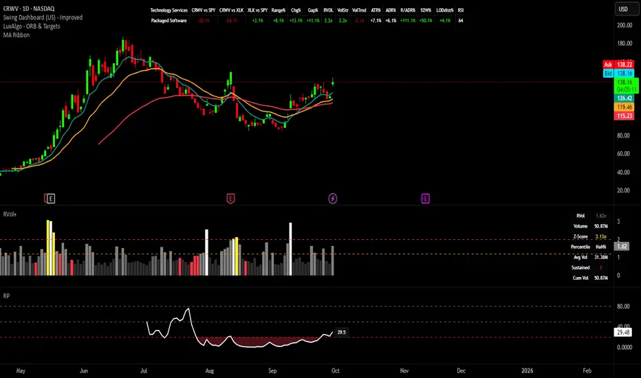
Swing Dashboard - Pro Trader Metrics with MTF & Enhanced VolumeDESCRIPTION:
A comprehensive real-time dashboard designed for swing traders and active investors trading US equities. Displays all critical metrics in one customizable panel overlay - no need to clutter your chart with multiple indicators.
KEY FEATURES:
📊 Relative Strength Analysis:
Stock vs Market (SPY/QQQ/IWM/DIA)
Stock vs Sector (automatic sector ETF detection)
Sector vs Market comparison
Customizable lookback period (5-60 days)
📈 Price & Range Metrics:
Daily range, change, and gap percentages
Distance from SMA20, SMA50, VWAP
52-week position percentage
ATR% and ADR% for volatility assessment
Range/ADR ratio for breakout detection
💪 Advanced Volume Analysis:
RVOL (full day volume vs 20-day average)
Volume Strength (bar-by-bar analysis)
Volume Trend (5-day vs 20-day momentum)
Customizable RVOL alert thresholds
Non-repainting volume calculations
⚙️ Multi-Timeframe (MTF) Mode:
View daily charts with 5-min or 15-min metric updates
Perfect for monitoring positions without switching timeframes
All calculations remain accurate across timeframes
🎨 Fully Customizable:
Choose which metrics to display
9 position options for the dashboard
Adjustable text size and colors
Toggle individual metrics on/off
Sector-specific ETF mapping for accurate RS calculations
TECHNICAL SPECIFICATIONS:
✅ Non-repainting - all calculations use confirmed bar data
✅ No lookahead bias or future data
✅ Optimized for US stocks with proper sector mapping
✅ Works on any timeframe (best on 5m-Daily)
✅ Pine Script v6 with best practices
✅ Handles edge cases and missing data gracefully
IDEAL FOR:
Swing traders monitoring multiple positions
Day traders needing quick metric overview
Investors tracking relative strength and momentum
Anyone who wants institutional-grade metrics in one place
SECTOR ETF MAPPING:
Automatically maps to correct sector ETFs: XLK, XLF, XLV, XLY, XLP, XLE, XLB, XLI, XLRE, XLC, XLU
HOW TO USE:
Green = Positive/Strong | Red = Negative/Weak | White = Neutral
RS > 0 = Outperforming benchmark/sector
RVOL > 1.5x = High volume day
VWAP% negative = Price below VWAP (mean reversion opportunity)
R/ADR > 100% = Extended range (potential exhaustion)
Perfect for traders who need professional-grade analysis without chart clutter.
TAGS:
dashboard, swing, relativestrengrh, sectoranalysis, volume, rvol, multitimeframe, mtf, tradingdashboard, metrics, daytrading, swingtrading, momentum, vwap, atr, volatility, volumeanalysis
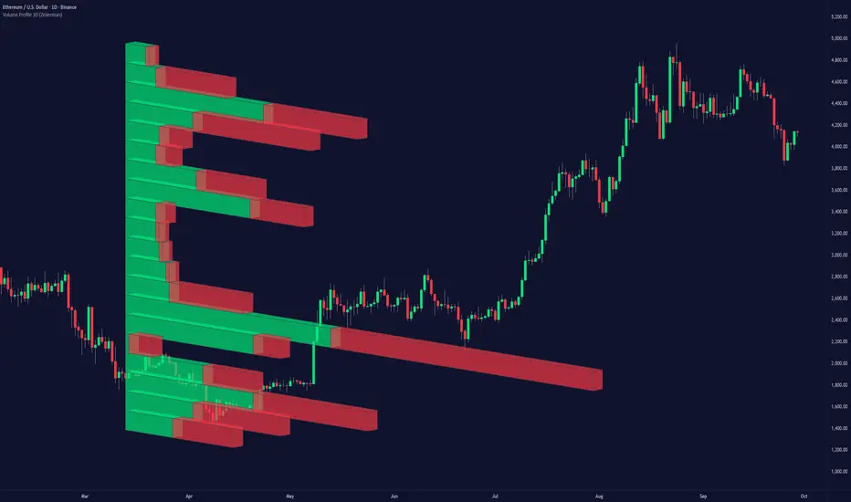
Volume Profile 3D (Zeiierman)█ Overview
Volume Profile 3D (Zeiierman) is a next-generation volume profile that renders market participation as a 3D-style profile directly on your chart. Instead of flat histograms, you get a depth-aware profile with parallax, gradient transparency, and bull/bear separation, so you can see where liquidity stacked up and how it shifted during the move.
Highlights:
3D visual effect with perspective and depth shading for clarity.
Bull/Bear separation to see whether up bars or down bars created the volume.
Flexible colors and gradients that highlight where the most significant trading activity took place.
This is a state-of-the-art volume profile — visually powerful, highly flexible, and unlike anything else available.
█ How It Works
⚪ Profile Construction
The price range (from highest to lowest) is divided into a number of levels (buckets). Each bar’s volume is added to the correct level, based on its average price. This builds a map of where trading volume was concentrated.
You can choose to:
Aggregate all volume at each level, or
Split bullish vs. bearish volume , slightly offset for clarity.
This creates a clear view of which price zones matter most to the market.
⚪ 3D Effect Creation
The unique part of this indicator is how the 3D projection is built. Each volume block’s width is scaled to its relative size, then tilted with a slope factor to create a depth effect.
maxVol = bins.bu.max() + bins.be.max()
width = math.max(1, math.floor(bucketVol / maxVol * ((bar_index - start) * mult)))
slope = -(step * dev) / ((bar_index - start) * (mult/2))
factor = math.pow(math.min(1.0, math.abs(slope) / step), .5)
width → determines how far the volume extends, based on relative strength.
slope → creates the angled projection for the 3D look.
factor → adjusts perspective to make deeper areas shrink naturally.
The result is a 3D-style volume profile where large areas pop forward and smaller areas fade back, giving you immediate visual context.
█ How to Use
⚪ Support & Resistance Zones (HVNs and Value Area)
Regions where a lot of volume traded tend to act like walls:
If price approaches a high-volume area from above, it may act as support.
From below, it may act as resistance.
Traders often enter or exit near these zones because they represent strong agreement among market participants.
⚪ POC Rejections & Mean Reversions
The Point of Control (POC) is the single price level with the highest volume in the profile.
When price returns to the POC and rejects it, that’s often a signal for reversal trades.
In ranging markets, price may bounce between edges of the Value Area and revert to POC.
⚪ Breakouts via Low-Volume Zones (LVNs)
Low volume areas (gaps in the profile) offer path of least resistance:
Price often moves quickly through these thin zones when momentum builds.
Use them to spot breakouts or continuation trades.
⚪ Directional Insight
Use the bull/bear separation to see whether buyers or sellers dominated at key levels.
█ Settings
Use Active Chart – Profile updates with visible candles.
Custom Period – Fixed number of bars.
Up/Down – Adjust tilt for the 3D angle.
Left/Right – Scale width of the profile.
Aggregated – Merge bull/bear volume.
Bull/Bear Shift – Separate bullish and bearish volume.
Buckets – Number of price levels.
Choose from templates or set custom colors.
POC Gradient option makes high volume bolder, low volume lighter.
-----------------
Disclaimer
The content provided in my scripts, indicators, ideas, algorithms, and systems is for educational and informational purposes only. It does not constitute financial advice, investment recommendations, or a solicitation to buy or sell any financial instruments. I will not accept liability for any loss or damage, including without limitation any loss of profit, which may arise directly or indirectly from the use of or reliance on such information.
All investments involve risk, and the past performance of a security, industry, sector, market, financial product, trading strategy, backtest, or individual's trading does not guarantee future results or returns. Investors are fully responsible for any investment decisions they make. Such decisions should be based solely on an evaluation of their financial circumstances, investment objectives, risk tolerance, and liquidity needs.
Intraday Rising & Reversal ScannerPine Script Description: Intraday Rising & Reversal ScannerThis Pine Script is a TradingView indicator designed to identify stocks with intraday (1-hour timeframe) potential for bullish (rising) or bearish (reversal) movements. It scans for stocks based on user-defined technical criteria, including price change, relative volume, RSI, EMA, ATR, and VWAP. The script plots signals on the chart, displays a summary table, and triggers alerts when conditions are met.FeaturesBullish Signal (Rising Stocks):1H Price Change: > 1% (configurable, e.g., >2% for volatile markets).
Relative Volume: > 2.0 (volume is at least twice the 20-period average).
RSI (14): Between 50 and 70 (strong but not overbought momentum).
Price vs EMA 13: Price above the 13-period EMA (confirms short-term uptrend).
ATR (14): Current ATR above its 20-period average (indicates volatility).
VWAP: Price above VWAP (optional, shown on chart for manual confirmation).
Bearish Signal (Reversal Stocks):1H Price Change: < -1% (configurable, e.g., <-2% for stronger reversals).
Relative Volume: > 2.0 (high volume confirms selling pressure).
RSI (14): > 70 (overbought, increasing reversal likelihood).
Price vs EMA 13: Price below the 13-period EMA (confirms short-term downtrend).
ATR (14): Current ATR above its 20-period average (indicates volatility).
VWAP: Price below VWAP (optional, shown on chart for manual confirmation).
Visualization:Bullish Signal: Green triangle below the bar.
Bearish Signal: Red triangle above the bar.
VWAP: Plotted as a blue line for manual verification.
Table: Displays real-time metrics (Change %, Relative Volume, RSI, Price vs EMA, ATR, VWAP) in the top-right corner, color-coded (green for bullish, red for bearish).
Alerts:Separate alerts for bullish ("Intraday Bullish Signal") and bearish ("Intraday Bearish Signal") conditions.
Customizable alert messages include parameter values for easy tracking.
How It WorksThe script runs on the 1-hour (1H) timeframe, ensuring all calculations are based on hourly data.
Indicators are computed:Change %: Percentage price change over the last hour.
Relative Volume: Current volume divided by the 20-period SMA of volume.
RSI: 14-period Relative Strength Index.
EMA 13: 13-period Exponential Moving Average.
ATR: 14-period Average True Range, compared to its 20-period SMA.
VWAP: Volume Weighted Average Price, plotted for visual confirmation.
Signals are generated when all conditions for either bullish or bearish criteria are met.
A table summarizes key metrics, and alerts can be set up for real-time notifications.
Usage InstructionsApply the Script:Open TradingView’s Pine Editor.
Copy and paste the script.
Click "Add to Chart" and set the chart to the 1-hour (1H) timeframe.
Set Up Alerts:Right-click on the chart > "Add Alert".
Select "Intraday Bullish Signal" or "Intraday Bearish Signal" as the condition.
Configure notifications (e.g., SMS, email, or TradingView alerts).
Manual VWAP Check:VWAP is plotted as a blue line. Verify that the price is above VWAP for bullish signals or below for bearish signals using the table or chart.
To make VWAP a mandatory filter, uncomment the VWAP conditions in the bull_signal and bear_signal definitions.
EMA-RSI-ADX Trend Bands
📌 EMA-RSI-ADX Trend Bands (ERA Trend Bands)
🔥 Overview
The ERA Trend Bands indicator combines Exponential Moving Average (EMA), Relative Strength Index (RSI), and Average Directional Index (ADX) into a powerful multi-factor trend system.
It helps traders:
Identify trend direction (Bullish / Bearish)
Measure trend strength using EMA deviation bands
Confirm momentum with RSI & ADX filters
Visualize conditions with dynamic colors, labels, tables, and signals
⚡ Key Features
📍 EMA Trend Bands
EMA100 with gradient glow effect showing trend bias
Strength bands around EMA (Very Weak → Hyper levels)
Bands color-coded for bullish/bearish extremes
📊 RSI + ADX Confluence
Bullish Signal: RSI ≥ threshold & ADX ≥ threshold → 🟢
Bearish Signal: RSI ≤ threshold & ADX ≤ threshold → 🔴
Candles recolored when conditions are met
Auto-generated labels show live RSI/ADX values
🧩 Strength Levels
Classifies deviation from EMA into 8 levels:
Neutral → Very Weak → Weak → Moderate → Strong → Very Strong → Extreme → Hyper
Dashboard table shows deviation % ranges & strength colors
Dynamic labels display Trend, Strength, Deviation %, RSI & ADX
🎨 Visual Enhancements
Gradient EMA line with glow effect
Bullish (greens) & bearish (reds) vibrant palettes
Background coloring (optional) based on strength
Symbols & labels for entry confirmation
🎯 How to Use
Trend Direction – EMA color + deviation bands show whether market is bullish or bearish.
Strength Confirmation – Use strength labels & dashboard table to gauge overextension.
Entry Signals – Watch for RSI/ADX confluence (green/red labels on chart).
Exits – Monitor when strength fades back toward Neutral/Weak levels.
⚙️ Settings & Inputs
EMA Settings → Length, Line Width, Gradient Intensity
RSI Settings → Length & Thresholds (Bullish / Bearish)
ADX Settings → Length & Thresholds (Bullish / Bearish)
Bands → Enable/disable EMA deviation bands
Labels/Table → Toggle strength info display
Colors → Fully customizable vibrant palettes
🚨 Alerts & Signals
Bullish Condition → RSI & ADX above thresholds
Bearish Condition → RSI & ADX below thresholds
Visual confirmation with labels, candles, and background
⚠️ Disclaimer
This script is for educational purposes only.
It does not constitute financial advice.
Always backtest and use proper risk management before trading live.
✨ Add EMA-RSI-ADX Trend Bands (ERA Trend Bands) to your chart to trade with clarity, strength, and precision.

Bollinger Bands (SMA 21, 2.618σ)Indicator Description: Bollinger Bands (2.618σ, 21 SMA) + RSI with Fibonacci
This custom indicator combines Bollinger Bands and Relative Strength Index (RSI), enhanced with Fibonacci-based configurations, to provide confluence signals for rejection candles, reversal setups, and continuation patterns.
Bollinger Bands Settings (Customized)
Middle Band → 21-period Simple Moving Average (SMA)
Upper Band → SMA + 2.618 standard deviations
Lower Band → SMA − 2.618 standard deviations
These parameters expand the bands compared to the traditional (20, 2.0) settings, making them better suited for volatility extremes and higher timeframe swing analysis.
Color Scheme
Middle Band = Orange
Upper Band = Red
Lower Band = Green
This color-coding emphasizes key rejection levels visually.
Candle Rejection Logic
The indicator is designed to highlight potential rejection candles when price interacts with the outer Bollinger Bands:
At the Upper Band, rejection signals suggest overextension and potential downside reaction.
At the Lower Band, rejection signals suggest oversold conditions and potential upside reaction.
Rejection Candle Types Tracked
Hammer (bullish reversal, lower rejection wick at bottom band)
Inverted Hammer (bearish reversal, upper rejection wick at top band)
Doji candles (indecision at band extremes)
Double Top formations near the upper band
Double Bottom formations near the lower band
Relative Strength Index (RSI) Settings
RSI is configured with Fibonacci retracement levels instead of traditional 30/70 thresholds.
Fibonacci sequence levels used include:
23.6% (0.236)
38.2% (0.382)
50% (0.5)
61.8% (0.618)
78.6% (0.786)
This alignment with Fibonacci ratios provides deeper market structure insights into momentum strength and exhaustion points.
Trading Confluence Zones
Upper Band + RSI at 0.618–0.786 zone → High probability bearish rejection.
Lower Band + RSI at 0.236–0.382 zone → High probability bullish reversal.
Band interaction + Doji or Hammer candles → Stronger signal confirmation.
Use Cases
Identifying trend exhaustion when price repeatedly fails to break above the upper band.
Spotting accumulation or distribution phases when price consolidates around Fibonacci-based RSI zones.
Detecting false breakouts when candle patterns (like Doji or Inverted Hammer) occur beyond the bands.
Why 2.618 Deviation & 21 SMA?
Standard Bollinger Bands (20, 2.0) capture ~95% of price action.
By widening to 2.618σ, we target extreme volatility outliers — areas where reversals are statistically more likely.
A 21-period SMA aligns better with common cycle lengths (3 trading weeks on daily charts) and Fibonacci-related time cycles.
Practical Strategy
Step 1: Watch when price touches or pierces the upper/lower band.
Step 2: Check for candle rejection patterns (Hammer, Inverted Hammer, Doji, Double Top/Bottom).
Step 3: Confirm with RSI Fibonacci levels for confluence.
Step 4: Trade with the prevailing trend or look for reversal setups if multiple confluence factors align.
Cautions
Not all touches of the bands signal reversals — strong trends can ride along the bands for extended periods.
Always combine with price action structure, volume, and higher timeframe trend bias.
📌 Summary
This indicator blends volatility-based bands with Fibonacci momentum analysis and classical candle rejection patterns. The combination of Bollinger Bands (21, 2.618σ) and RSI Fibonacci levels helps traders detect high-probability rejection zones, reversal opportunities, and overextended conditions with improved accuracy over traditional default settings.

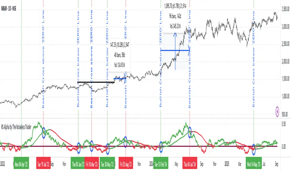
RS Alpha by The Noiseless TraderRS Alpha by The Noiseless Trader plots a clean, benchmark‑relative strength line for any symbol and (optionally) a mean line to assess trend and momentum in relative performance. It’s designed for uncluttered, professional RS analysis and works across any timeframe.
Compare any symbol vs a benchmark (default: NSE:NIFTY).
Optional log‑normalized RS for return‑aware comparisons.
Optional RS Mean with trend coloring (rising/falling).
Optional RS Trend zero‑line coloring based on short‑range slope.
Lightweight alerts for rising/falling RS mean.
Tip: Use RS to identify leaders (RS > 0 with rising mean) and laggards (RS < 0 with falling mean), then align setups with your price action rules.
Reading the indicator
Leadership: RS > 0 and RS Mean rising → outperformance vs benchmark.
Weakness: RS < 0 and RS Mean falling → underperformance vs benchmark.
Inflections: Watch RS crossing above/below its Mean for early shifts.
Zero‑line context: With RS Trend on, the zero line subtly reflects short‑term slope (green for positive, maroon for negative).
Alerts
Rising Strength – RS Mean turning/remaining upward.
Declining Strength – RS Mean turning/remaining downward.
(Use these as context; execute entries on your price‑action rules.)
Best practices
Pair RS with your trend/structure rules (e.g., higher highs + RS leadership).
For sectors/baskets, keep the Comparative Symbol consistent to rank peers.
Log‑normalized RS helps when comparing assets with very different volatilities or large base effects.
Test multiple length and Mean settings; 60 is a balanced default for swing/positional work.
Credits
Original concept & code: © bharatTrader
Modifications & refinements: The Noiseless Trader
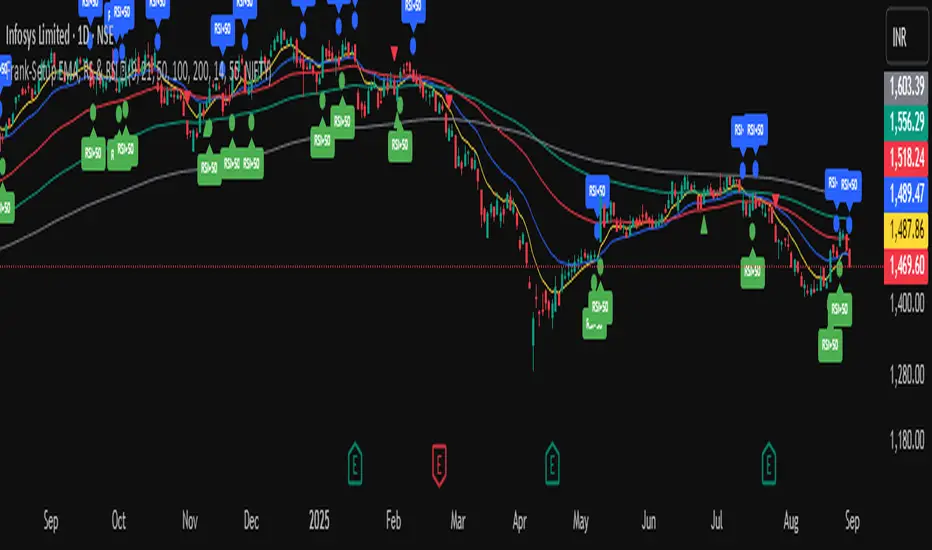
Frank-Setup EMA, RS & RSI ✅It is a clean and simple indicator designed to identify weakness in stocks using two proven methods: RSI and Relative Strength (RS) vs. a benchmark (e.g., NIFTY).
🔹 Features
RSI Weakness Signals
Plots when RSI crosses below 50 (weakness begins).
Plots when RSI moves back above 50 (weakness ends).
Relative Strength (RS) vs Benchmark
Compares stock performance to a chosen benchmark.
Signals when RS drops below 1 (stock underperforming).
Signals when RS recovers above 1 (strength resumes).
Clear Visual Markers
Circles for RSI signals.
Triangles for RS signals.
Optional RSI labels for clarity.
Built-in Alerts
Get notified instantly when RSI or RS weakness starts or ends.
No need to constantly watch charts.
🎯 Use Case
This tool is built for traders who want to:
Spot shorting opportunities when a stock shows weakness.
Track underperformance vs. the index.
Manage risk by exiting longs when weakness appears.
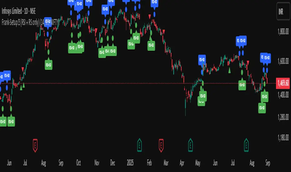
Frank-Setup ✅ (RSI + RS only)Frank-Shorting Setup ✅ is an indicator designed to help traders spot weakness in a stock by combining RSI and Relative Strength (RS) analysis.
🔹 Key Features
RSI Weakness Signals
Marks when RSI falls below 50 (downside pressure begins).
Marks when RSI moves back above 50 (weakness ends).
Relative Strength (RS) vs Benchmark
Compares stock performance to a benchmark (e.g., NIFTY).
Signals when RS drops below 1 (stock underperforming).
Signals when RS moves back above 1 (strength resumes).
Clear Chart Markings
Circles for RSI signals.
Triangles for RS signals.
Optional labels for extra clarity.
Alerts Built-In
Get notified when RSI or RS weakness starts/ends.
No need to monitor charts all the time

Frank-Shorting Setup ✅ (RSI + RS only)An indicator designed to help traders spot weakness in a stock by combining RSI and Relative Strength (RS) analysis.
🔹 Key Features
RSI Weakness Signals
Marks when RSI falls below 50 (downside pressure begins).
Marks when RSI moves back above 50 (weakness ends).
Relative Strength (RS) vs Benchmark
Compares stock performance to a benchmark (e.g., NIFTY).
Signals when RS drops below 1 (stock underperforming).
Signals when RS moves back above 1 (strength resumes).
Clear Chart Markings
Circles for RSI signals.
Triangles for RS signals.
Optional labels for extra clarity.
Alerts Built-In
Get notified when RSI or RS weakness starts/ends.
No need to monitor charts all the time
MSTY-WNTR Rebalancing SignalMSTY-WNTR Rebalancing Signal
## Overview
The **MSTY-WNTR Rebalancing Signal** is a custom TradingView indicator designed to help investors dynamically allocate between two YieldMax ETFs: **MSTY** (YieldMax MSTR Option Income Strategy ETF) and **WNTR** (YieldMax Short MSTR Option Income Strategy ETF). These ETFs are tied to MicroStrategy (MSTR) stock, which is heavily influenced by Bitcoin's price due to MSTR's significant Bitcoin holdings.
MSTY benefits from upward movements in MSTR (and thus Bitcoin) through a covered call strategy that generates income but caps upside potential. WNTR, on the other hand, provides inverse exposure, profiting from MSTR declines but losing in rallies. This indicator uses Bitcoin's momentum and MSTR's relative strength to signal when to hold MSTY (bullish phases), WNTR (bearish phases), or stay neutral, aiming to optimize returns by switching allocations at key turning points.
Inspired by strategies discussed in crypto communities (e.g., X posts analyzing MSTR-linked ETFs), this indicator promotes an active rebalancing approach over a "set and forget" buy-and-hold strategy. In simulated backtests over the past 12 months (as of August 4, 2025), the optimized version has shown potential to outperform holding 100% MSTY or 100% WNTR alone, with an illustrative APY of ~125% vs. ~6% for MSTY and ~-15% for WNTR in one scenario.
**Important Disclaimer**: This is not financial advice. Past performance does not guarantee future results. Always consult a financial advisor. Trading involves risk, and you could lose money. The indicator is for educational and informational purposes only.
## Key Features
- **Momentum-Based Signals**: Uses a Simple Moving Average (SMA) on Bitcoin's price to detect bullish (price > SMA) or bearish (price < SMA) trends.
- **RSI Confirmation**: Incorporates MSTR's Relative Strength Index (RSI) to filter signals, avoiding overbought conditions for MSTY and oversold for WNTR.
- **Visual Cues**:
- Green upward triangle for "Hold MSTY".
- Red downward triangle for "Hold WNTR".
- Yellow cross for "Switch" signals.
- Background color: Green for MSTY, red for WNTR.
- **Information Panel**: A table in the top-right corner displays real-time data: BTC Price, SMA value, MSTR RSI, and current Allocation (MSTY, WNTR, or Neutral).
- **Alerts**: Configurable alerts for holding MSTY, holding WNTR, or switching.
- **Optimized Parameters**: Defaults are tuned (SMA: 10 days, RSI: 15 periods, Overbought: 80, Oversold: 20) based on simulations to reduce whipsaws and capture trends effectively.
## How It Works
The indicator's logic is straightforward yet effective for volatile assets like Bitcoin and MSTR:
1. **Primary Trigger (Bitcoin Momentum)**:
- Calculate the SMA of Bitcoin's closing price (default: 10-day).
- Bullish: Current BTC price > SMA → Potential MSTY hold.
- Bearish: Current BTC price < SMA → Potential WNTR hold.
2. **Secondary Filter (MSTR RSI Confirmation)**:
- Compute RSI on MSTR stock (default: 15-period).
- For bullish signals: If RSI > Overbought (80), signal Neutral (avoid overextended rallies).
- For bearish signals: If RSI < Oversold (20), signal Neutral (avoid capitulation bottoms).
3. **Allocation Rules**:
- Hold 100% MSTY if bullish and not overbought.
- Hold 100% WNTR if bearish and not oversold.
- Neutral otherwise (e.g., during choppy or extreme markets) – consider holding cash or avoiding trades.
4. **Rebalancing**:
- Switch signals trigger when the hold changes (e.g., from MSTY to WNTR).
- Recommended frequency: Weekly reviews or on 5% BTC moves to minimize trading costs (aim for 4-6 trades/year).
This approach leverages Bitcoin's influence on MSTR while mitigating the risks of MSTY's covered call drag during downtrends and WNTR's losses in uptrends.
## Setup and Usage
1. **Chart Requirements**:
- Apply this indicator to a Bitcoin chart (e.g., BTCUSD on Binance or Coinbase, daily timeframe recommended).
- Ensure MSTR stock data is accessible (TradingView supports it natively).
2. **Adding to TradingView**:
- Open the Pine Editor.
- Paste the script code.
- Save and add to your chart.
- Customize inputs if needed (e.g., adjust SMA/RSI lengths for different timeframes).
3. **Interpretation**:
- **Green Background/Triangle**: Allocate 100% to MSTY – Bitcoin is in an uptrend, MSTR not overbought.
- **Red Background/Triangle**: Allocate 100% to WNTR – Bitcoin in downtrend, MSTR not oversold.
- **Yellow Switch Cross**: Rebalance your portfolio immediately.
- **Neutral (No Signal)**: Panel shows "Neutral" – Hold cash or previous position; reassess weekly.
- Monitor the panel for key metrics to validate signals manually.
4. **Backtesting and Strategy Integration**:
- Convert to a strategy script by changing `indicator()` to `strategy()` and adding entry/exit logic for automated testing.
- In simulations (e.g., using Python or TradingView's backtester), it has outperformed buy-and-hold in volatile markets by ~100-200% relative APY, but results vary.
- Factor in fees: ETF expense ratios (~0.99%), trading commissions (~$0.40/trade), and slippage.
5. **Risk Management**:
- Use with a diversified portfolio; never allocate more than you can afford to lose.
- Add stop-losses (e.g., 10% trailing) to protect against extreme moves.
- Rebalance sparingly to avoid over-trading in sideways markets.
- Dividends: Reinvest MSTY/WNTR payouts into the current hold for compounding.
## Performance Insights (Simulated as of August 4, 2025)
Based on synthetic backtests modeling the last 12 months:
- **Optimized Strategy APY**: ~125% (by timing switches effectively).
- **Hold 100% MSTY APY**: ~6% (gains from BTC rallies offset by downtrends).
- **Hold 100% WNTR APY**: ~-15% (losses in bull phases outweigh bear gains).
In one scenario with stronger volatility, the strategy achieved ~4533% APY vs. 10% for MSTY and -34% for WNTR, highlighting its potential in dynamic markets. However, these are illustrative; real results depend on actual BTC/MSTR movements. Test thoroughly on historical data.
## Limitations and Considerations
- **Data Dependency**: Relies on accurate BTC and MSTR data; delays or gaps can affect signals.
- **Market Risks**: Bitcoin's volatility can lead to false signals (whipsaws); the RSI filter helps but isn't perfect.
- **No Guarantees**: This indicator doesn't predict the future. MSTR's correlation to BTC may change (e.g., due to regulatory events).
- **Not for All Users**: Best for intermediate/advanced traders familiar with ETFs and crypto. Beginners should paper trade first.
- **Updates**: As of August 4, 2025, this is version 1.0. Future updates may include volume filters or EMA options.
If you find this indicator useful, consider leaving a like or comment on TradingView. Feedback welcome for improvements!

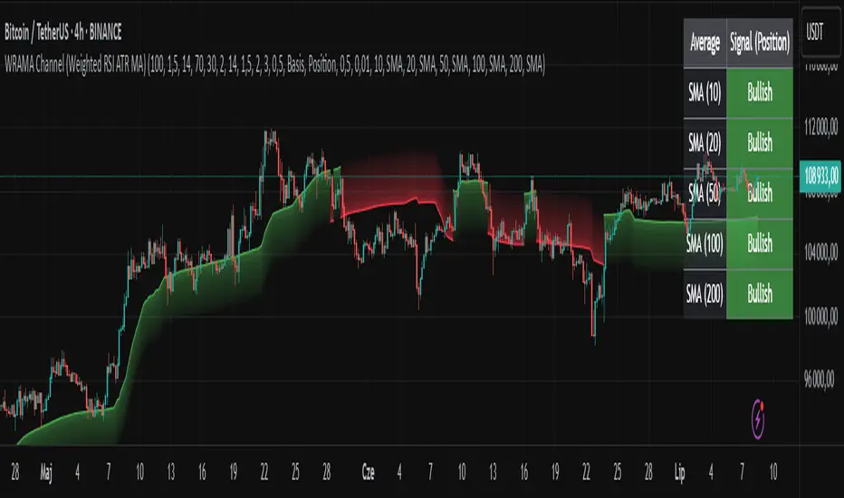
WRAMA Channel (Weighted RSI ATR MA)OVERVIEW
The WRAMA Channel (Weighted RSI ATR MA) is an advanced technical analysis tool designed to react more quickly to price movements compared to indicators using conventional moving averages. It combines the Relative Strength Index (RSI), Average True Range (ATR), and a weighted moving average, resulting in the WRAMA. This indicator forms a dynamic price channel based on a weighted average that incorporates both trend strength (via RSI) and market volatility (via ATR). It helps traders identify trends, potential reversals, and breakout signals, while offering broad customization options.
Key Features
WRAMA Price Channel:
Generates a dynamic channel around the weighted moving average (WRAMA), adapting to market volatility and momentum, similar to Bollinger Bands. Users are encouraged to adjust channel width and length according to their strategy.
The upper and lower channel bands are calculated based on a percentage deviation from the baseline line.
The channel fill color changes depending on the price's position relative to the baseline (green above, red below), with an optional gradient for better visualization.
Weighted Moving Average (WRAMA):
WRAMA is a custom weighted moving average (MA1), where closing prices are weighted based on RSI and ATR, allowing it to dynamically adapt to market conditions.
Baseline: The WRAMA line calculated over a user-defined period.
WRAMA Calculation:
RSI Weight: Based on RSI value. When RSI is in extreme zones (below the lower threshold or above the upper threshold), an extreme weight is applied. Otherwise, the weight is based on the squared RSI value divided by 100, raised to a power defined by the rsi_weight_factor.
ATR Weight: Based on the ATR-to-average-ATR ratio. If ATR exceeds a threshold (atr_threshold × avg_atr), an extreme weight is applied. Otherwise, the weight is based on the squared ratio of ATR to average ATR, raised to the power of the atr_weight_factor.
Combined Weight: RSI and ATR weights are combined using a rsi_atr_balance parameter. Final weight = RSI weight × balance + ATR weight × (1 - balance).
WRAMA Calculation: The closing price is multiplied by the combined weight. The result is averaged over the ma_length period and divided by the average of the weights, forming the WRAMA line. For current WRAMA (ma_length = 1), the calculation simplifies to a single weighted price.
Additional Moving Averages:
For additional confirmations, the indicator supports up to five moving averages (MA1–MA5) with various types (SMA, EMA, WMA, HMA, ALMA) and customizable periods.
All additional MAs are calculated based on WRAMA or its baseline, ensuring consistency and enabling deeper analysis within a unified methodology. MA trend directions can be tracked in a built-in signal table.
Trading Signals:
Breakout Signals: Breakouts above/below the channel are optionally marked with triangle shapes (green for bullish, red for bearish).
MA Signals: Price position relative to MAs or their slope generates bullish/bearish signals. These are optionally visualized with default triangles (green up, red down).
A signal table in the top-right corner summarizes the status of each moving average – bullish, bearish, or neutral.
Customization Options
Channel Settings:
MA Period: Length of the WRAMA baseline (default: 100).
Channel Deviation : Percentage offset from the baseline for upper/lower bands (default: 1.5%).
RSI Settings:
RSI Period: Length of the RSI calculation (default: 14).
RSI Upper/Lower Threshold: Overbought/oversold levels (default: 70/30).
RSI Weight Factor: Influence of RSI on weighting (default: 2.0).
ATR Settings:
ATR Period: ATR calculation length (default: 14).
ATR Threshold: Volatility threshold as a multiple of average ATR (default: 1.5).
ATR Weight Factor: Influence of ATR on weighting (default: 2.0).
RSI & ATR Combined:
Extreme Weight: Weight applied in extreme RSI/ATR conditions (default: 3.0).
RSI/ATR Balance: Balance between RSI and ATR influence (default: 0.5).
Signal Settings:
Show Breakout Signals: Enable/disable breakout triangles.
Show MA Signals: Enable/disable MA-based signals.
MA Signal Source: Choose between current WRAMA or baseline.
MA Signal Analysis: Based on price position or slope.
Neutral Threshold : Minimum distance from MA for signal neutrality (default: 0.5%).
Minimum MA Slope : Minimum slope for trend direction signals (default: 0.01%).
Moving Averages (MA1–MA5):
Options to enable/disable, select type (SMA, EMA, WMA, HMA, ALMA), set period length, and choose color.
Style Settings:
Gradient Fill: Enable/disable gradient coloring within the channel.
Show Baseline: Enable/disable WRAMA baseline visibility.
Colors: Customize line, fill, and signal colors.
Use Cases
Trend Identification: The WRAMA channel highlights trend direction and potential reversal zones when price contacts the channel edges.
Breakout Signals: Channel breakouts may indicate trend shifts or momentum surges.
MA Analysis: The signal table provides a clear summary of market direction (bullish, bearish, or neutral) based on selected moving averages.
Trading Strategies: Suitable for trend-following, mean-reversion, and scalping strategies, depending on user preferences and settings.
Notes
The indicator offers a high degree of flexibility, making it adaptable to various trading styles, instruments, and timeframes.
It is recommended to adjust channel length and width to fit your trading strategy.
Backtesting settings on historical data is advised to optimize parameters for a specific strategy and market.
CAN INDICATORCAN Moving Averages Indicator - Feature Guide
1. Multiple Moving Averages (20 MAs)
- Supports up to 20 individual moving averages
- Each MA can be independently configured:
- Enable/Disable toggle
- Length (period) setting
- Type selection (SMA, EMA, DEMA, VWMA, RMA, WMA)
- Color customization
- Individual timeframe settings when global timeframe is disabled
Pre-configured MA Settings:
1. MA1-8: SMA type
- Lengths: 20, 50, 100, 200, 365, 489, 600, 1460
2. MA9-20: EMA type
- Lengths: 30, 60, 120, 240, 300, 400, 500, 700, 800, 900, 1000, 2000
2. Global Timeframe Settings
Location: Global Settings group
Features:
- Use Global Timeframe: Toggle to use one timeframe for all MAs
- Global Timeframe: Select the timeframe to apply globally
3. Label Display Options
Location: Main Inputs section
Controls:
- Show MA Type: Display MA type (SMA, EMA, etc.)
- Show MA Length: Display period length
- Show Resolution: Display timeframe
- Label Offset: Adjust label position
4. Cross Alerts System
Location: Cross Alerts group
Features:
1. Price Crosses:
- Alerts when price crosses any selected MA
- Select MA to monitor (1-20)
- Triggers on crossover/crossunder
2. MA Crosses:
- Alerts when one MA crosses another
- Select fast MA (1-20)
- Select slow MA (1-20)
- Triggers on crossover/crossunder
5. Relative Strength (RS) Analysis
Location: Relative Strength group
Features:
- Select any MA to monitor (1-20)
- Compares MA to its own average
- Adjustable RS Length (default 14)
- Visual feedback via background color:
- Green: MA above its average (uptrend)
- Red: MA below its average (downtrend)
- Customizable colors and transparency
6. Moving Average Types Available
1. **SMA** (Simple Moving Average)
- Equal weight to all prices
2. **EMA** (Exponential Moving Average)
- More weight to recent prices
3. **DEMA** (Double Exponential Moving Average)
- Reduced lag compared to EMA
4. **VWMA** (Volume Weighted Moving Average)
- Incorporates volume data
5. **RMA** (Running Moving Average)
- Smoother than EMA
6. **WMA** (Weighted Moving Average)
- Linear weight distribution
Usage Tips
1. **For Trend Following:**
- Enable longer-period MAs (MA4-MA8)
- Use cross alerts between long-term MAs
- Monitor RS for trend strength
2. **For Short-term Trading:**
- Focus on shorter-period MAs (MA1-MA3, MA9-MA11)
- Enable price cross alerts
- Use multiple timeframe analysis
3. **For Multiple Timeframe Analysis:**
- Disable global timeframe
- Set different timeframes for each MA
- Compare MA relationships across timeframes
4. **For Performance:**
- Disable unused MAs
- Limit active alerts to necessary pairs
- Use RS selectively on key MAs
